email: zerbini@astbo1.bo.cnr.it
Tide gauges measure sea-level changes as variations in the relative position between the crust and the ocean surface. These measurements are difficult to interpret because they are influenced by several phenomena inducing vertical crustal movements. At present, vertical crustal motions at tide gauges can be measured to high accuracy independently of the sea-level reference surface by means of space techniques, therefore it will be possible to separate the crustal motions from the absolute sea-level variations. Tide gauge measurements are difficult to compare because tide gauges are referred to local reference systems and they have not yet been connected on a common datum. However, it should be pointed out that several international efforts are underway both at global (IOC, 1990) and regional scales which aim to overcome this problem. Nowadays, space geodesy techniques provide the possibility to connect tide gauges on a common datum by measuring via GPS their position to subcentimeter accuracy with respect to a well defined geocentric reference system such as the one, for example, established by the global network of Satellite Laser Ranging (SLR)/Very Long Baseline Interferometry (VLBI) fiducial stations. Moreover, it is available the International Terrestrial Reference System (ITRS) which has been established through an ensamble of SLR, VLBI, Global Positioning System (GPS) and Lunar Laser Ranging (LLR) stations (Boucher and Altamimi, 1993a, 1993b). The use of the ITRS has been recommended by the Commission on Mean Sea Level and Tides of the International Association for the Physical Sciences of the Ocean (IAPSO) in their well known Woods Hole report (Carter et al., 1989) and in the more recent report of the Surrey Workshop (Carter, 1994).
The SELF (SEa Level Fluctuations: geophysical interpretation and environmental impact) project, approved by ILP and financed by the Commission of the European Communities within the framework of the Environment program and developed in the time frame 1990-1992, was a pilot study (Zerbini et al., 1991) which provided a fundamental contribution to a better understanding of global change by providing a necessary base to succesfully approach the measurement of sea level fluctuations and to reliably assess the factors causing sea level rise. It involved several Institutions in 4 member states of the Community (Italy, Fed. Rep. of Germany, Greece and United Kingdom), Switzerland and Poland. The Institutions worked together to achieve the following objectives: to select, in the Mediterranean region, fiducial reference stations and well established tide gauges and to provide GPS links between the (SLR/VLBI) fiducial stations of the global network and the tide gauges; to improve GPS measurement procedures by using Water Vapor Radiometers to reduce vertical uncertainties to 1 cm or less; to perform measurements of absolute-g both at fiducial sites and tide gauges to monitor, with an independent system, vertical surface elevation changes; to perform, in selected areas of the Mediterranean basin, observations of geologic sea level markers of the past; to collect, analyze and interpret tide gauge data; to develop realistic models for tidal loading and tectonics in the Mediterranean region; to define corrections for the Earth's surface deformation due to exogenic causes and to study long-term variability of relative sea level.
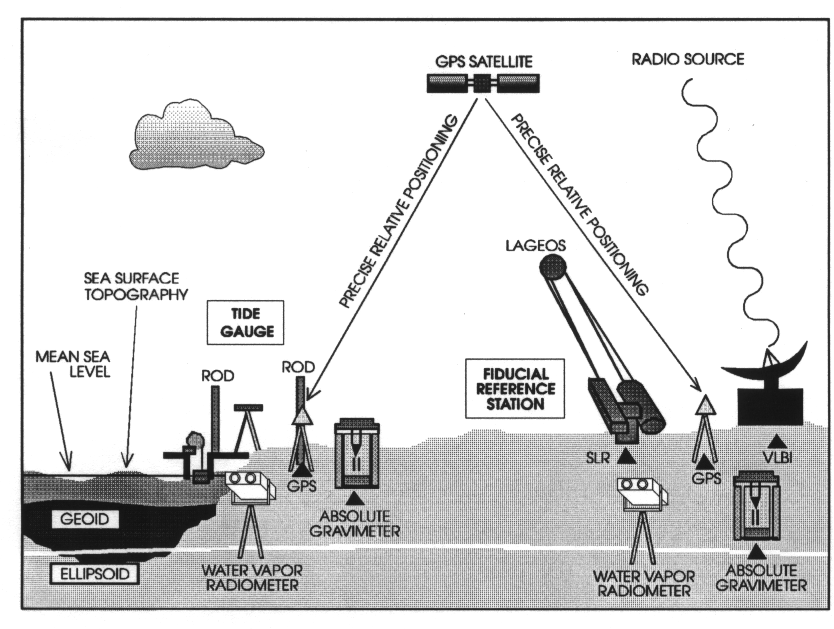
Figure 1 illustrates schematically the measuring approach which has been adopted in the SELF project. Tide gauge measurements are referred to a permanent shore mark, the Tide Gauge BenchMark (TGBM). Simultaneous GPS observations were performed to tie the TGBM and the selected fiducial stations of the global reference system. Whenever the TGBM proved not to be suitable for GPS observations a new benchmark was installed and linked to the TGBM by means of high precision levelling. The global reference system adopted is the one provided by the SLR/GPS solution SSC(DUT)94C01R derived by the Delft University of Technology (Noomen et al., 1994). Several campaigns were carried out to link the selected tide gauges to the nearest fiducial reference station all across the Mediterranean basin from the Straits of Gibraltar as far as the Black Sea (Figure 2).
Simultaneous observations at tide gauges and reference stations were performed by using dual-frequency GPS receivers for, at least, 48 hours continuously with a sampling rate of 30 seconds. Simultaneously with GPS observations, two dual-frequency ground-based, transportable Water Vapor Radiometers (WVR) have been used in France, Italy and Greece to improve the estimation of the tropospheric path delay due to the water vapor content in the atmosphere. In the analysis, the WVR data have been combined with the GPS data in order to determine the station height to the best achiavable accuracy. Table 1 lists the GPS marker height in the SSC(DUT)94C01R reference system, the height difference between the GPS benchmark and the TGBM measured by means of high precision levelling, and finally the TGBM in the adopted reference.
Table 1. GPS benchmark height and TGBM height in the SSC(DUT)94C01R reference system, Height difference between the GPS benchmark and the TGBM.
Tide gauge site  GPS marker height   Height difference   TGBM height
                 in the SLR              GPS-TGBM (m)    in the SLR
                 SSC(DUT)94C01R                          SSC(DUT94C01R
                 ref. system (m)                         ref.system (m)

Brindisi         42.648 +-  0.005    0.667 +-  0.001     41.981 +-  0.005
Catania          51.977     0.009    9.007     0.002     42.970     0.009
Pt. Corsini      39.820     0.006  -0.536     0.001     40.356     0.006
Venice           44.629     0.014  -2.031     0.002     46.660     0.014
Trieste          52.981     0.006    7.451     0.002     45.530     0.006
Genoa            49.306     0.002    2.518     0.002     46.788     0.003
Marseille        61.753     0.003   11.204     0.001     50.549     0.003
Preveza          28.403     0.007    0.525     0.001     27.878     0.007
Patrai           28.406     0.008    1.374     0.002     27.032     0.008
Kalamai          26.976     0.013    0.007     0.001     26.969     0.013
Soudhas          38.968     0.017   14.735     0.002     24.233     0.017
Piraieus         39.660     0.004    0.644     0.001     39.016     0.004
Siros            40.028     0.005    0.411     0.002     39.617     0.005
Katakolon        28.071     0.003    3.709     0.002     24.362     0.004
Rhodos           29.184     0.003    7.265     0.002     21.919     0.004
Iraklion         27.356     0.008    1.909     0.003     25.447     0.009
Katsively        30.467     0.007    5.685     0.002     24.782     0.007
Tuapse           18.722     0.004    0.000     0.000     18.725     0.004
Algeciras        44.537     0.003   -0.471     0.002     45.008     0.004
Tarifa           46.524     0.002    2.691     0.002     43.833     0.003
Cadiz            52.295     0.005    3.317     0.002     48.978     0.005
Ceuta            44.887     0.003   -0.673     0.002     45.560     0.004
Gibraltar        45.520     0.003   -0.480     0.002     46.000     0.004
Absolute gravity has also been measured both at the tide gauges and at
the reference sites (Table 2). The average precision of the measurements of
absolute g is in the order of 1.5 �gal; since the free-air vertical gradient of g is
equal to 3 �gal/cm it is possible to detect changes in gravity due to pure height
variations of the order of 1 cm, which is comparable with the precision of the
height determinations achieved with the GPS technique. The combination of space
geodetic measurements and absolute g observations can therefore provide a
vertical datum accurate to, at least, the 1 cm level which is a necessary requisite
in order to be able to detect and control sea level fluctuations most likely induced
by global warming and to separate this signal from that which might be originated
by tectonic movements or exogenic forces. Table 2. Absolute gravity values.
Site           Epoch           g          sigma      h0
                           (microgal)   (microgal)   (m)

Basovizza      1991.85     980 568 052     0.8     0.903
Matera         1991.85     980 185 527     0.9     0.925
Medicina       1992.85     980 473 607     1.5     0.916
Medicina       1995.10     980 474 790     1.6     0.900
Marseille      1993.40     980 485 131     1.2     0.931
Grasse         1993.40     980 216 056    0.9     0.929
Noto           1993.50     979 992 652     1.5     0.948
Genoa          1993.40     980 558 119     1.0     0.931
Venice         1994.95     980 635 142     3.2     0.000
Naples         1994.40     980 257 805     4.0     0.982
Pt. Corsini    1995.10     980 483 313    11.5    0.950
Brindisi       1994.95     980 293 481    3.0     0.000
Catania        1994.85     980 044 166    3.5     0.000
Karitsa        1993.90     979 913 519     1.3     0.920
Askites        1993.85     980 250 029     1.0     0.935
Ermoupoli      1993.85     980 048 152     2.0     0.951
Katakolon      1993.85     979 897 950     2.1     0.948
Xrisokellaria  1993.85     979 854 674     0.7     0.942
Kattavia       1993.85     979 861 917     0.7     0.939
Roumelli       1993.75     979 827 682     0.9     0.947
Dionysos       1993.75     979 961 222     1.8     0.943
San Fernando   1994.20     979 826 339     3.5     1.312
Tarifa         1994.20     979 737 252     3.8     1.323
Ceuta          1994.20     979 755 018     3.1     1.318
Simeiz         1994.45     980 566 746    12.4     1.307
Tuapse         1994.45     980 542 128    28.2     1.316
Zelenchukskaya 1994.45     980 249 154     2.6     1.306
Baksan         1994.45     979 909 691     2.6     1.316
Modelling the sea level decadal variations can improve the local trend
estimates or even allow for a detection of an anthropogenic acceleration in the
trend. Furthermore, interannual to decadal fluctuation in sea-level may in itself
prove useful as an effective indicator of climate changes. A substantial fraction of
the intraannual to decadal fluctations in coastal sea-level is non-steric and forced
mechanically by the atmosphere. To some extent, coastal sea-level integrates over
the atmospheric forcing, thus enhancing the long-period part over shorter periods.
Thus, studies of the interannual fluctuations in coastal sea-level may reveal
changes in the mechanical forcing of the atmosphere, i.e. in the regional
atmospheric circulation, that cannot be detected directly from the meteorological
data. Analysis of the tide gauge data has been performed in the framework of the
SELF project. Mixed quality tide gauge data are available for the Mediterranean
Sea. Although trend values can easily be assigned, the analysis indicates that
records at least 40 years long should be used if errors less than 0.5 mm/yr are
required. The analyses of the monthly sea level data reveal an unexpectedly large
variability on the coastal seasonal tidal constituent which is spatially highly
coherent. This variability on dacadal time scales most likely is associated with
changes in the regional atmospheric circulation. The trends determined from the longer RLR records available in the Mediterranean are compiled in Table 3 together with the relative sea-level rise expected from isostatic compensation due to post-glacial rebound. In the Mediterranean, this effect is of the order 0.3 mm/a. Thus, at tectonically stable sites we should expect a relative sea-level rise close to the global one.
To improve local trend estimations from shorter records a better understanding of the response of sea level to the various forcing parameters is needed. Hydrodynamical models to simulate sea-level variability due to meteorological forcing and steric effects would be an appropriate tool to separate these effects from the long-term sea-level changes. However, in the absence of such models, other means can be utilized, which are based on the assumption, that the interannual to multidecadal sea-level variability is spatially coherent within properly defined regions. Thus, in regions, where a long and qualitatively good record is available, this record may be used as "base record''. For shorter records, trends are estimated from the differences of monthly (or annual) means to the base record thus eliminating the synchroneous part of the sea-level variations (Sj�berg, 1987). For the western part of the Mediterranean, Marseille is a potential base station, while Trieste could serve as such for the eastern part. The trends determined with Marseille as base station tend to be slightly larger than those using Trieste (Table 3). Especially for records spanning the end of the last and the beginning of the present century (marked with an asterisk in Table 3), Trieste introduces a negative bias, which may be due to the small overlap of these records with Trieste. For records spanning the second half of the century, both Marseille and Trieste as base records improve the trends in the sense that the interstation scatter is reduced. At one of the two records at Split (Rt. Mar.), the effects of using Trieste and Marseille are opposite, possibly indicating some data problems. As it can be seen from Table 3, at least at the tide gauges included in the present study, crustal movements are small compared to the decadal to multidecadal sea- level variability discussed above but of the same order as the long-term trend in sea level, thus necessitating a careful monitoring if crustal movement is to be separated from the oceanographic contribution to relative sea-level changes.
Table 3. Local trends in relative sea level.
The stations are sorted according to the available data. N: number of available monthly sea-level values, t: sea-level trend in mm/a, sigmat: standard error in mm/a, tP: trend due to postglacial rebound as computed with the ICE-3G model (Peltier and Tushingham, 1989), tTr/tMa: trends in mm/a determined using Trieste and Marseille, respectively, as base record. For records marked with an asterisk, the overlap with Trieste is small, explaining the large differences compared to the trends derived with Marseille as base station. rC: crustal movement rates (positive for uplift) decontaminated for post-glacial rebound effects; these rates given are calculated from rC = -(tMa - tP - e), where e is the eustatic sea-level change. We assumed e = 1.8 mm/a (Douglas, 1992).
Station         Begin  End    N     t  sigmat   tP   tTr  tMa      rC

Marseille      1885  1989  1157   1.1  0.1   -0.2  1.03  1.10    0.5
Genova          1884  1988  994   1.3  0.1   -0.2  0.98  1.21    0.5
Trieste        1905  1990  960   1.1  0.2   -0.3  1.10  1.17    0.3
Lagos          1908  1989  863   1.4  0.2   -0.4  1.39  1.42    0.0
Tuapse         1917  1990  844   2.2  0.3   -0.1  1.99  2.17   -0.3
Bakar          1930  1990  600   0.9  0.3   -0.3  1.04  1.69   -0.2
Split Rt Mar.  1952  1990  450   0.1  0.5   -0.3 -1.29  0.73    0.8
Split Harbour   1954  1990    44  -0.8  0.5   -0.3 -0.05  1.46    0.0
Cagliari       1896  1934  433   1.3  0.4    0.2  1.15  1.74    0.3
Rovinj         1955  1990  424  -0.2  0.5   -0.3  0.57  2.21   -0.7
Dubrovnik      1956  1990  419  -0.1  0.5   -0.3  0.58  2.10   -0.6
Alicante II    1960  1987  332  -1.4  0.4   -0.3 -0.18  1.15    0.3
Koper          1962  1990  332  -0.5  0.6   -0.3  1.07  2.21   -0.7
Bar            1964  1990   18   1.4  0.7         2.57  3.25
P. Maurizio    1896  1922  309   1.1  0.6   -0.1  1.52  2.71 * -1.0
Civitavecchia  1896  1922  304   1.2  0.7    0.0  0.59  1.43 *  0.4
Alicante I     1952  1987   303  -2.2  0.4   -0.3 -2.71 -0.24    1.7
Napoli (Man.)   1896  1922  301   2.1  0.7    0.0  2.18  3.25 * -1.5
Palermo         1896  1922  294   1.0  0.7    0.3 -1.39  1.15 *  0.9
Venezia (S.St.) 1896  1920  288   4.4  1.2   -0.3  2.11  4.72 * -3.2
Port Said      1923  1946  287   4.7  1.0         5.20  4.20
Venezia (Ars.)  1889  1913  287   1.8  1.4   -0.3  3.58  4.60 * -3.1
Gibraltar      1961  1989  272  -0.7  0.8   -0.6  0.24  0.15    1.0
Napoli (Ars.)  1899  1922  263   2.5  1.5    0.0  1.94  3.00 * -1.2
Porto Corsini  1969  1972    45  -3.1             17.99 -0.97
References
Boucher C. and Z. Altamimi, 1993a. Development of a Conventional Terrestrial Reference Frame. In Contributions of Space Geodesy to Geodynamics: Earth Dynamics, American Geophysical Union, Geodynamics Series, 24:89-97.
Boucher C. and Z. Altamimi, 1993b. Contribution of IGS92 to the TRF. In proceedings of 1993 IGS workshop, Bern, March 25-26, 1993, 175-183.
Carter W.E., D.G. Aubrey, T. Baker, C. Boucher, C. LeProvost, D. Pugh, W.R. Peltier, M. Zumberge, R.H. Rapp, R.E. Schutz, K.O. Emery and D.B. Enfield, 1989. Geodetic fixing of tide gauge bench marks, Technical Report, CRC-89-5, Coastal Research Center, WHOI-89-31, pp. 46.
Carter W.E. (Edt.), 1994. Report of the Surrey Workshop of the IAPSO Tide Gauge Bench Mark Fixing Committee. Deacon Laboratory, Godalming, Surrey, United Kingdom, December 13-15, 1993, NOAA Technical Report NOSOES0006.
Douglas B.C., 1992. Global sea level acceleration. Journ. Geophys. Res., 97:12699 - 12706.
IOC, 1990. Global Sea Level Observing System (GLOSS): Implementation Plan, Intergovernamental Oceanographic Commission, Technical Series, 35, Unesco, pp. 90.
Noomen R., T.A. Springer, B.A.C. Ambrosius, K. Herzberger, D.C. Kuijper, G.J. Mets, B. Overgaauw and K.F. Wakker, 1994. Crustal deformations in the Mediterranean area computed from SLR and GPS observations, sumitted to Journal of Geodynamics.
Peltier W.R. and A.M. Tushingham, 1989. Global Sea Level Rise and the Greenhouse Effect: Might They Be Connected? Science, 244:806-810.
Sjoberg L.E., 1987. Comparison of some methods of determining land uplift rates from tide gauge data. ZfV, 2:69-73.
Zerbini S., T. Baker, H.G. Kahle, G. Veis and P. Wilson, 1991. SEa-Level Fluctuations: geophysical interpretation and environmental impact (SELF). Proposal submitted to the Commission of the European Communities for the Environment Programme, pp. 50.